The followings introductory post is intended for new users of R. It deals with the restructuring of data: what it is and how to perform it using base R functions and the {reshape} package.
This is a guest article by Dr. Robert I. Kabacoff, the founder of (one of) the first online R tutorials websites: Quick-R. Kabacoff has recently published the book ”R in Action“, providing a detailed walk-through for the R language based on various examples for illustrating R’s features (data manipulation, statistical methods, graphics, and so on…). The previous guest post by Kabacoff introduced data.frame objects in R.

Let us now talk about the Aggregation and Restructuring of data in R:

Aggregation and Restructuring
R provides a number of powerful methods for aggregating and reshaping data. When you aggregate data, you replace groups of observations with summary statistics based on those observations. When you reshape data, you alter the structure (rows and columns) determining how the data is organized. This article describes a variety of methods for accomplishing these tasks.
We’ll use the mtcars data frame that’s included with the base installation of R. This dataset, extracted from Motor Trend magazine (1974), describes the design and performance characteristics (number of cylinders, displacement, horsepower, mpg, and so on) for 34 automobiles. To learn more about the dataset, see help(mtcars).
Transpose
The transpose (reversing rows and columns) is perhaps the simplest method of reshaping a dataset. Use the t() function to transpose a matrix or a data frame. In the latter case, row names become variable (column) names. An example is presented in the next listing.
Listing 1 Transposing a dataset
1 2 3 4 5 6 7 8 9 10 11 12 13 14 | > cars <- mtcars[1:5,1:4] > cars mpg cyl disp hp Mazda RX4 21.0 6 160 110 Mazda RX4 Wag 21.0 6 160 110 Datsun 710 22.8 4 108 93 Hornet 4 Drive 21.4 6 258 110 Hornet Sportabout 18.7 8 360 175 > t(cars) Mazda RX4 Mazda RX4 Wag Datsun 710 Hornet 4 Drive Hornet Sportabout mpg 21 21 22.8 21.4 18.7 cyl 6 6 4.0 6.0 8.0 disp 160 160 108.0 258.0 360.0 hp 110 110 93.0 110.0 175.0 |
Listing 1 uses a subset of the mtcars dataset in order to conserve space on the page. You’ll see a more flexible way of transposing data when we look at the reshape package later in this article.
Aggregating data
It’s relatively easy to collapse data in R using one or more by variables and a defined function. The format is
1 | aggregate(x, by, FUN) |
where x is the data object to be collapsed, by is a list of variables that will be crossed to form the new observations, and FUN is the scalar function used to calculate summary statistics that will make up the new observation values.
As an example, we’ll aggregate the mtcars data by number of cylinders and gears, returning means on each of the numeric variables (see the next listing).
Listing 2 Aggregating data
1 2 3 4 5 6 7 8 9 10 11 12 13 | > options(digits=3) > attach(mtcars) > aggdata <-aggregate(mtcars, by=list(cyl,gear), FUN=mean, na.rm=TRUE) > aggdata Group.1 Group.2 mpg cyl disp hp drat wt qsec vs am gear carb 1 4 3 21.5 4 120 97 3.70 2.46 20.0 1.0 0.00 3 1.00 2 6 3 19.8 6 242 108 2.92 3.34 19.8 1.0 0.00 3 1.00 3 8 3 15.1 8 358 194 3.12 4.10 17.1 0.0 0.00 3 3.08 4 4 4 26.9 4 103 76 4.11 2.38 19.6 1.0 0.75 4 1.50 5 6 4 19.8 6 164 116 3.91 3.09 17.7 0.5 0.50 4 4.00 6 4 5 28.2 4 108 102 4.10 1.83 16.8 0.5 1.00 5 2.00 7 6 5 19.7 6 145 175 3.62 2.77 15.5 0.0 1.00 5 6.00 8 8 5 15.4 8 326 300 3.88 3.37 14.6 0.0 1.00 5 6.00 |
In these results, Group.1 represents the number of cylinders (4, 6, or ![]() and Group.2 represents the number of gears (3, 4, or 5). For example, cars with 4 cylinders and 3 gears have a mean of 21.5 miles per gallon (mpg).
and Group.2 represents the number of gears (3, 4, or 5). For example, cars with 4 cylinders and 3 gears have a mean of 21.5 miles per gallon (mpg).
When you’re using the aggregate() function , the by variables must be in a list (even if there’s only one). You can declare a custom name for the groups from within the list, for instance, using by=list(Group.cyl=cyl, Group.gears=gear).
The function specified can be any built-in or user-provided function. This gives the aggregate command a great deal of power. But when it comes to power, nothing beats the reshape package.
The reshape package
The reshape package is a tremendously versatile approach to both restructuring and aggregating datasets. Because of this versatility, it can be a bit challenging to learn.
We’ll go through the process slowly and use a small dataset so that it’s clear what’s happening. Because reshape isn’t included in the standard installation of R, you’ll need to install it one time, using install.packages(“reshape”).
Basically, you’ll “melt” data so that each row is a unique ID-variable combination. Then you’ll “cast” the melted data into any shape you desire. During the cast, you can aggregate the data with any function you wish. The dataset you’ll be working with is shown in table 1.
Table 1 The original dataset (mydata)
ID | Time | X1 | X2 |
| 1 | 1 | 5 | 6 |
| 1 | 2 | 3 | 5 |
| 2 | 1 | 6 | 1 |
| 2 | 2 | 2 | 4 |
In this dataset, the measurements are the values in the last two columns (5, 6, 3, 5, 6, 1, 2, and 4). Each measurement is uniquely identified by a combination of ID variables (in this case ID, Time, and whether the measurement is on X1 or X2). For example, the measured value 5 in the first row is uniquely identified by knowing that it’s from observation (ID) 1, at Time 1, and on variable X1.
Melting
When you melt a dataset, you restructure it into a format where each measured variable is in its own row, along with the ID variables needed to uniquely identify it. If you melt the data from table 1, using the following code
1 2 | library(reshape) md <- melt(mydata, id=(c("id", "time"))) |
You end up with the structure shown in table 2.
Table 2 The melted dataset
ID | Time | Variable | Value |
| 1 | 1 | X1 | 5 |
| 1 | 2 | X1 | 3 |
| 2 | 1 | X1 | 6 |
| 2 | 2 | X1 | 2 |
| 1 | 1 | X2 | 6 |
| 1 | 2 | X2 | 5 |
| 2 | 1 | X2 | 1 |
| 2 | 2 | X2 | 4 |
Note that you must specify the variables needed to uniquely identify each measurement (ID and Time) and that the variable indicating the measurement variable names (X1 or X2) is created for you automatically.
Now that you have your data in a melted form, you can recast it into any shape, using the cast() function.
Casting
The cast() function starts with melted data and reshapes it using a formula that you provide and an (optional) function used to aggregate the data. The format is
1 | newdata <- cast(md, formula, FUN) |
Where md is the melted data, formula describes the desired end result, and FUN is the (optional) aggregating function. The formula takes the form
1 | rowvar1 + rowvar2 + … ~ colvar1 + colvar2 + … |
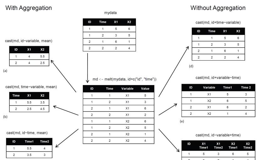
In this formula, rowvar1 + rowvar2 + … define the set of crossed variables that define the rows, and colvar1 + colvar2 + … define the set of crossed variables that define the columns. See the examples in figure 1. (click to enlarge the image)
Figure 1 Reshaping data with the melt() and cast() functions
Because the formulas on the right side (d, e, and f) don’t include a function, the data is reshaped. In contrast, the examples on the left side (a, b, and c) specify the mean as an aggregating function. Thus the data are not only reshaped but aggregated as well. For example, (a) gives the means on X1 and X2 averaged over time for each observation. Example (b) gives the mean scores of X1 and X2 at Time 1 and Time 2, averaged over observations. In (c) you have the mean score for each observation at Time 1 and Time 2, averaged over X1 and X2.
As you can see, the flexibility provided by the melt() and cast() functions is amazing. There are many times when you’ll have to reshape or aggregate your data prior to analysis. For example, you’ll typically need to place your data in what’s called long format resembling table 2 when analyzing repeated measures data (data where multiple measures are recorded for each observation).
Summary
Chapter 5 of R in Action reviews many of the dozens of mathematical, statistical, and probability functions that are useful for manipulating data. In this article, we have briefly explored several ways of aggregating and restructuring data.
This article first appeared as chapter 5.6 from the “R in action“ book, and is published with permission from Manning publishing house. Other books in this serious which you might be interested in are (see the beginning of this post for a discount code):
- Machine Learning in Action by Peter Harrington
- Gnuplot in Action (Understanding Data with Graphs) by Philipp K. Janert


I’m afraid I can’t read figure 1. even clicking on it gets stuck. and there was I hoping to master the cast function!
The image loads fine now.
After melting data and merging in a new id variabl I want to cast the data frame back into the original form with the addition of this new id var….My situation is very similar to the one in the figure (d) in this article except I added the new id var after melting..
However when I try to do this even though I do not include a function it assigns length as default. THis is not the behaviour predicted in this article and I am trying to figure out what is going wron.
thanks
[email protected]
We have what we think is a code problem with the aggregate(), aggregate.formula method. How can we send you our sample data and step by step walk-through? Is this the right place? Thanks, Alan
Hi Alan,
I suspect stackoverflow.com is a better place for such questions.