Analyzing coverage of R unit tests in packages – the {testCoverage} package

(guest post by Andy Nicholls and the team of Mango Business Solutions)

Introduction

Testing is a crucial component in ensuring that the correct analyses are deployed. However it is often considered unglamorous; a poor relation in terms of the time and resources allocated to it in the process of developing a package. But with the increasing popularity and commercial application of R it testing is a subject that is gaining significantly in importance.

At the time of writing there are 5987 packages on CRAN. Due to the nature of CRAN and the motivations of contributors the quality of packages can vary greatly. Some are very popular and well maintained, others are essentially inactive with development having all but ceased. As the number of packages on CRAN continues to grow, determining which packages are fit for purpose in a commercial environment is becomming an increasingly difficult task. There have been numerous articles and blog posts on the subject of CRAN’s growth and the quality of R packages. In particular, Francis Smart’s R-bloggers post entitled Does R have too many packages? highlights five perceived concerns with the growing number of R packages. I would like to expand on one of these themes in particular, namely the “inconsistent quality of individual packages”.

There are many ways in which a package can be assessed for quality. Popularity is clearly one: if lots of people use it then it must be quite good! But popular packages tend to also have authors that actively develop their packages and fix bugs as users identify them. Development activity is therefore another factor; the length of time that a package has existed for; the package dependency tree and the number of reverse ‘Depends’, ‘Imports’ and ‘Suggests’; the number of authors and their reputation; and finally there is testing. Francis briefly mentions testing in his post noting that “testing is still largely left up to the authors and users”. In other words there is no requirement for an author to write tests for their package and often they don’t!

Continue reading “Analyzing coverage of R unit tests in packages – the {testCoverage} package”

Simpler R coding with pipes > the present and future of the magrittr package

Background

It has only been 7 months and a bit since my initial magrittr commit to GitHub on January 1st. It has had more success than I had anticipated, and it appears that I was not quite alone with a frustration which caused me to start the magrittr project. I am not easily frustrated with R, but after a few weeks working with F# at work, I felt it upon returning to R: I had gotten used to writing code in a different way — all nicely aligned with thought and order of execution. The forward pipe operator |> was so addictive that being unable to do something similar in R was more than mildly irritating. Reversing thought, deciphering nested function calls, and making excessive use of temporary variables almost became deal breakers! Surprisingly, I had never really noticed this before, but once I did my returning to R became a difficult crossing.

An amazing thing about R is that it is a very flexible language and the problem could be solved. The |> operator in F# is indeed very simple: it is defined as let (|>) x f = f x. However, the usefulness of this simplicity relies heavily on a concept that is not available in Rpartial application. Furthermore, functions in F# almost always adhere to certain design principles which make the simple definition sufficient. Suppose that f is a function of two arguments, then in F# you may apply f to only the first argument and obtain a new function as the result — a function of the second argument alone. This is partial application, and works with any number of arguments, but application is always from left to right in the argument list. This is why the most important argument (and the one most likely to be a left-hand side object in the pipeline) is almost always the last argument, which in turn makes the simple definition of |> work. To illustrate, consider the following example:

some_value |> some_function other_value

Here, some_function is partially applied to other_value, creating a new function of a single argument, and by the simple definition of |>, this is applied to some_value.

It was clear to me that because R is lacking native partial application and conventions on argument order, no simple solution would be satisfactory, although definitely possible, see e.g. here or here. I wanted to make something that would feel natural in R, and which would serve the main purpose of improving cognitive performance of those writing the code, and of those reading the code.

It turned out that while I was working on magrittr’s %>% operator, Hadley Wickham and Romain Francois was implementing a similar %.% operator in their dplyr package which they announced on January 17. However, it was not quite as flexible, and we thought that piping functionality was better placed in its own more light-weight package. Hadley joined the magrittr project, and in dplyr 2.0 the %.% operator was deprecated — instead%>% was imported from magrittr.

Continue reading “Simpler R coding with pipes > the present and future of the magrittr package”

The dendextend package for visualizing and comparing trees of hierarchical clusterings (slides from useR!2014)

When using the dendextend package in your work, please cite it using:

Tal Galili (2015). dendextend: an R package for visualizing, adjusting, and comparing trees of hierarchical clustering. Bioinformatics. doi:10.1093/bioinformatics/btv428

This week I presented in the useR!2014 my package dendextend (also on github), for easily manipulating, visualizing, and comparing dendrograms. Put simply, it is a package designed to easily create figures like these:

2015-06-28 20_58_26-Clipboard

Here is my presentation from useR:

[gview file=”https://www.r-statistics.com/wp-content/uploads/2014/07/2014-07-01-useR2014-03.pdf” profile=”null” save=”1″]

You are also invited to give a look to the current version of the package vignettes:

https://github.com/talgalili/dendextend/blob/master/vignettes/dendextend-tutorial.pdf

I highly welcome features suggestions and bug reports (or just “wow, this is awesome”) sent to my e-mail (tal.galili AT gmail.com), you can also leave a comment or use the github issue page.

A sidenote on useR!2014: this year’s useR conference was wonderful! I enjoyed the many talks, sessions, posters, and especially the so many wonderful R users I got to meet (and I will not try to list all of you – but you know who you are, and how much I enjoyed seeing you!). As corny as it may sound – we, the people who use R, are truly a community. There is a lot to be said about getting to meet so many people who share my own passion for statistical programming, open source, collaboration, open science, and a better future in general. Gladly, you can get a sense of what happened there by having a look at the twitter hashtag #useR2014. Several great R bloggers already started writing about it, you can see their posts here: 1, 2, 3, 4, 5. And I hope more posts will follow. I hope to see you in next year’s useR!2015!

R 3.0.2 and RStudio 0.9.8 are released!

R 3.0.2 (codename “Frisbee Sailing”) was released yesterday. The full list of new features and bug fixes is provided below.

Also, RStudio v0.98 (in a “secret” preview) was announced two days ago with MANY new features, including:

Upgrading to R 3.0.2

You can download the latest version from here. Or, if you are using Windows, you can upgrade to the latest version using the installr package (also available on CRAN and github). Simply run the following code:

# installing/loading the package:
if(!require(installr)) {
install.packages("installr"); require(installr)} #load / install+load installr

updateR(to_checkMD5sums = FALSE) # the use of to_checkMD5sums is because of a slight bug in the MD5 file on R 3.0.2. This issue is already resolved in the installr version on github, and will be released into CRAN in about a month from now..

I try to keep the installr package updated and useful. If you have any suggestions or remarks on the package, you’re invited to leave a comment below.

If you use the global library system (as I do), you can run the following in the new version of R:

source("https://www.r-statistics.com/wp-content/uploads/2010/04/upgrading-R-on-windows.r.txt")
New.R.RunMe()

p.s: you can also use the installr package to quickly install the new RStudio by using:

# installing/loading the package:
if(!require(installr)) {
install.packages("installr"); require(installr)} #load / install+load installr

install.RStudio()

Continue reading “R 3.0.2 and RStudio 0.9.8 are released!”

A speed test comparison of plyr, data.table, and dplyr

ssssssspeed_521872450_d085d1e928

Guest post by Jake Russ

For a recent project I needed to make a simple sum calculation on a rather large data frame (0.8 GB, 4+ million rows, and ~80,000 groups). As an avid user of Hadley Wickham’s packages, my first thought was to use plyr. However, the job took plyr roughly 13 hours to complete.

plyr is extremely efficient and user friendly for most problems, so it was clear to me that I was using it for something it wasn’t meant to do, but I didn’t know of any alternative screwdrivers to use.

I asked for some help on the manipulator Google group , and their feedback led me to data.table and dplyr, a new, and still in progress, package project by Hadley.

What follows is a speed comparison of these three packages incorporating all the feedback from the manipulator folks. They found it informative, so Tal asked me to write it up as a reproducible example.

Continue reading “A speed test comparison of plyr, data.table, and dplyr”

Analyzing Your Data on the AWS Cloud (with R)

Guest post by Jonathan Rosenblatt

Disclaimer:
This post is not intended to be a comprehensive review, but more of a “getting started guide”. If I did not mention an important tool or package I apologize, and invite readers to contribute in the comments.

Introduction

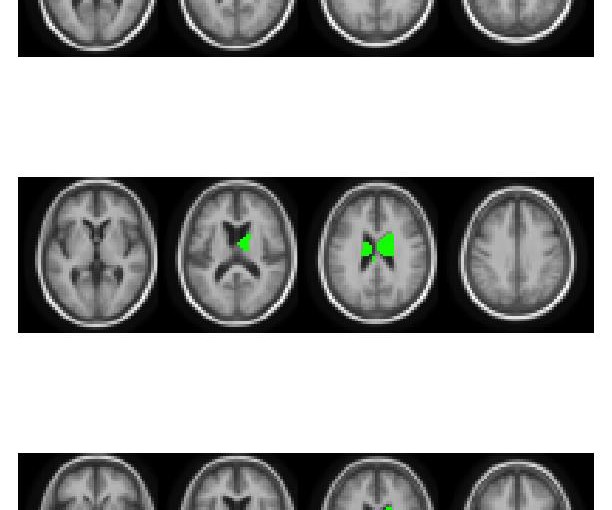
I have recently had the delight to participate in a “Brain Hackathon” organized as part of the OHBM2013 conference. Being supported by Amazon, the hackathon participants were provided with Amazon credit in order to promote the analysis using Amazon’s Web Services (AWS). We badly needed this computing power, as we had 14*109 p-values to compute in order to localize genetic associations in the brain leading to Figure 1.

Figure 1- Brain volumes significantly associated to genotype.
brain_image01

While imaging genetics is an interesting research topic, and the hackathon was a great idea by itself, it is the AWS I wish to present in this post. Starting with the conclusion: 

Storing your data and analyzing it on the cloud, be it AWSAzureRackspace or others, is a quantum leap in analysis capabilities. I fell in love with my new cloud powers and I strongly recommend all statisticians and data scientists get friendly with these services. I will also note that if statisticians do not embrace these new-found powers, we should not be surprised if data analysis becomes synonymous with Machine Learning and not with Statistics (if you have no idea what I am talking about, read this excellent post by Larry Wasserman).

As motivation for analysis in the cloud consider:

  1. The ability to do your analysis from any device, be it a PC, tablet or even smartphone.
  2. The ability to instantaneously augment your CPU and memory to any imaginable configuration just by clicking a menu. Then scaling down to save costs once you are done.
  3. The ability to instantaneously switch between operating systems and system configurations.
  4. The ability to launch hundreds of machines creating your own cluster, parallelizing your massive job, and then shutting it down once done.

Here is a quick FAQ before going into the setup stages.

FAQ

Q: How does R fit in?

Continue reading “Analyzing Your Data on the AWS Cloud (with R)”

Tailor Your Tables with stargazer: New Features for LaTeX and Text Output

Guest post by Marek Hlavac

Since its first introduction on this blog, stargazer, a package for turning R statistical output into beautiful LaTeX and ASCII text tables, has made a great deal of progress. Compared to available alternatives (such as apsrtable or texreg), the latest version (4.0) of stargazer supports the broadest range of model objects. In particular, it can create side-by-side regression tables from statistical model objects created by packages AER, betareg, dynlm, eha, ergm, gee, gmm, lme4, MASS, mgcv, nlme, nnet, ordinal, plm, pscl, quantreg, relevent, rms, robustbase, spdep, stats, survey, survival and Zelig.  You can install stargazer from CRAN in the usual way:

install.packages(“stargazer”)

New Features: Text Output and Confidence Intervals

In this blog post, I would like to draw attention to two new features of stargazer that make the package even more useful:

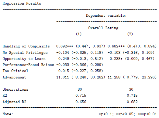
  • stargazer can now produce ASCII text output, in addition to LaTeX code. As a result, users can now create beautiful tables that can easily be inserted into Microsoft Word documents, published on websites, or sent via e-mail. Sharing your regression results has never been easier. Users can also use this feature to preview their LaTeX tables before they use the stargazer-generated code in their .tex documents.
  • In addition to standard errors, stargazer can now report confidence intervals at user-specified confidence levels (with a default of 95 percent). This possibility might be especially appealing to researchers in public health and biostatistics, as the reporting of confidence intervals is very common in these disciplines.

In the reproducible example presented below, I demonstrate these two new features in action.


Reproducible Example

I begin by creating model objects for two Ordinary Least Squares (OLS) models (using the lm() command) and a probit model (using glm() ). Note that I use data from attitude, one of the standard data frames that should be provided with your installation of R.

## 2 OLS models

linear.1 <- lm(rating ~ complaints + privileges + learning + raises + critical, data=attitude)
linear.2 <- lm(rating ~ complaints + privileges + learning, data=attitude)

## create an indicator dependent variable, and run a probit model

attitude$high.rating <- (attitude$rating > 70)
probit.model <- glm(high.rating ~ learning + critical + advance, data=attitude, family = binomial(link = "probit"))

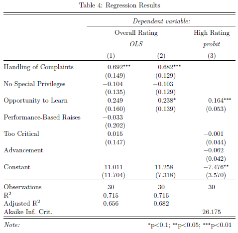
I then use stargazer to create a ‘traditional’ LaTeX table with standard errors. With the sole exception of the argument no.space – which I use to save space by removing all empty lines in the table – both the command call and the resulting table should look familiar from earlier versions of the package:

stargazer(linear.1, linear.2, probit.model, title="Regression Results", align=TRUE, dep.var.labels=c("Overall Rating","High Rating"), covariate.labels=c("Handling of Complaints","No Special Privileges", "Opportunity to Learn","Performance-Based Raises","Too Critical","Advancement"), omit.stat=c("LL","ser","f"), no.space=TRUE)

table_example_1

Continue reading "Tailor Your Tables with stargazer: New Features for LaTeX and Text Output"

Top 100 R packages for 2013 (Jan-May)!

What are the top 100 (most downloaded) R packages in 2013? Thanks to the recent release of RStudio of their “0-cloud” CRAN log files (but without including downloads from the primary CRAN mirror or any of the 88 other CRAN mirrors), we can now answer this question (at least for the months of Jan till May)!

By relying on the nice code that Felix Schonbrodt recently wrote for tracking packages downloads, I have updated my installr R package with functions that enables the user to easily download and visualize the popularity of R packages over time. In this post I will share some nice plots and quick insights that can be made from this great data. The code for this analysis is given at the end of this post.

Top 8 most downloaded R packages – downloads over time

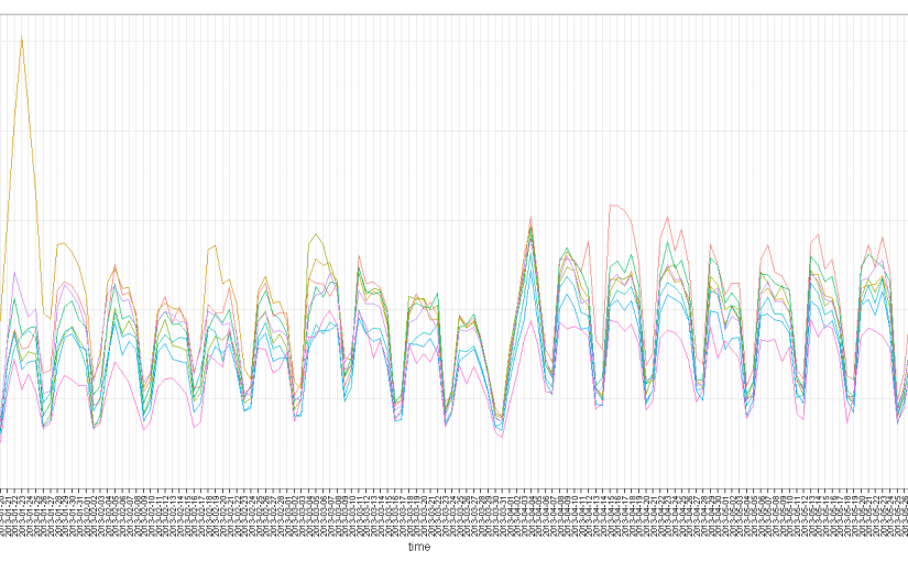
Let’s first have a look at the number of downloads per day for these 5 months, of the top 8 most downloaded packages (click the image for a larger version):

top_8_R_Packages_over_time

We can see the strong weekly seasonality of the downloads,  with Saturday and Sunday having much fewer downloads than other days. This is not surprising since we know that the countries which uses R the most have these days as rest days (see James Cheshire’s world map of R users). It is also interesting to note how some packages had exceptional peaks on some dates. For example, I wonder what happened on January 23rd 2013 that the digest package suddenly got so many downloads, or that colorspace started getting more downloads from April 15th 2013.

“Family tree” of the top 100 most downloaded R packages

We can extract from this data the top 100 most downloaded R packages. Moreover, we can create a matrix showing for each package which of our unique ids (censored IP addresses), has downloaded which package. Using this indicator matrix, we can thing of the “similarity” (or distance) between each two packages, and based on that we can create a hierarchical clustering of the packages – showing which packages “goes along” with one another.

With this analysis, you can locate package on the list which you often use, and then see which other packages are “related” to that package.  If you don’t know that package – consider having a look at it – since other R users are clearly finding the two packages to be “of use”.

Such analysis can (and should!) be extended. For example, we can imagine creating a “suggest a package” feature based on this data, utilizing the package which you use, the OS that you use, and other parameters.  But such coding is beyond the scope of this post.

Here is the “family tree” (dendrogram) of related packages:

Family_tree_of_Top_100_R_Packages

To make it easier to navigate, here is a table with links to the top 100 R packages, and their links:

Continue reading “Top 100 R packages for 2013 (Jan-May)!”

Answering "How many people use my R package?"

The question “How many people use my R package?” is a natural question that (I imagine) every R package developer asks himself at some point or another. After many years in the dark, a silver lining has now emerged thanks to the good people at RStudio. Just yesterday, a blog post by Hadley Wickham was written about the newly released CRAN log files of the RStudio cloud CRAN!

Already out, and the R blogosphere started buzzing with action: James Cheshire created a beautiful world map which highlights the countries based on how much people there use of R. Felix Schonbrodt wrote a great post on Tracking CRAN packages downloads. In the meantime, I’ve started crafting some basic functions for package developers to easily check how many users downloaded their package. These functions are now available on the installr package github page.

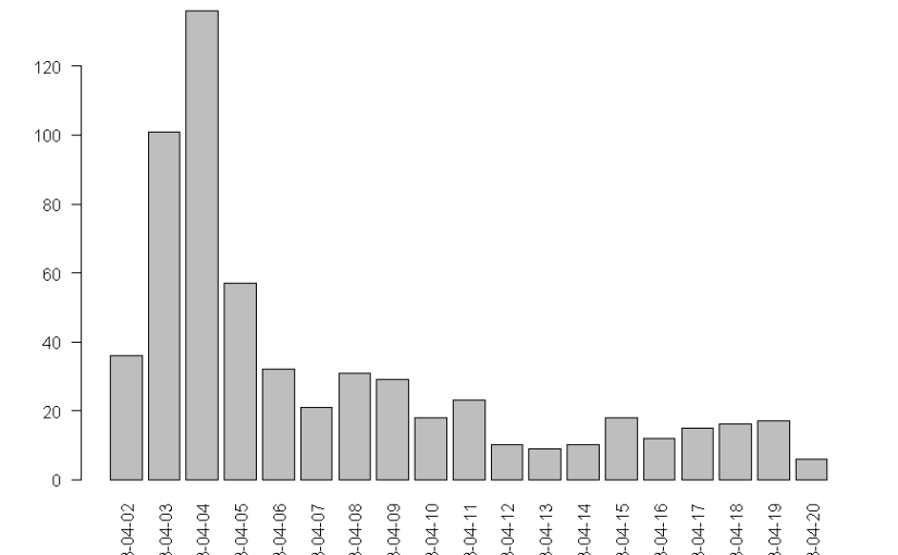
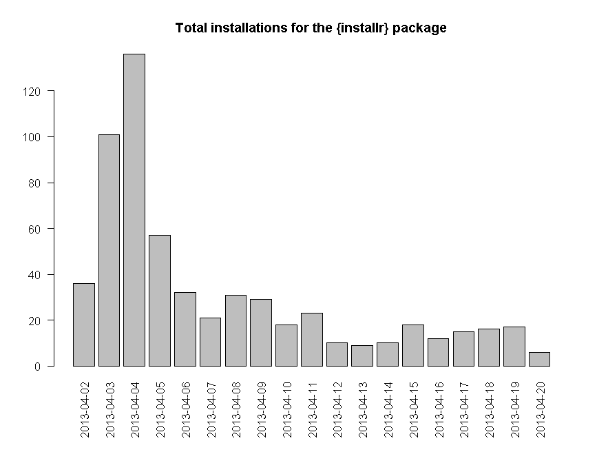
Here is the output for the number of unique ips who downloaded the installr package around the time R 3.0.0 was released (click to see a larger image):

installr_installations_per_day

And here is the code to allow you to make a similar plot for the package which interests you:

# if (!require('devtools')) install.packages('devtools'); require('devtools')
# make sure you have Rtools installed first! if not, then run:
#install_Rtools()
#install_github('installr', 'talgalili') # get the latest installr R package
# or run the code from here:
# https://github.com/talgalili/installr/blob/master/R/RStudio_CRAN_data.r

if(packageVersion("installr") %in% c("0.8","0.9","0.9.2")) install.packages('installr') #If you have one of the older installr versions, install the latest one....

require(installr)

# The first two functions might take a good deal of time to run (depending on the date range)
RStudio_CRAN_data_folder <- download_RStudio_CRAN_data(START = '2013-04-02', END = '2013-04-05') # around the time R 3.0.0 was released
my_RStudio_CRAN_data <- read_RStudio_CRAN_data(RStudio_CRAN_data_folder)

 # barplots: (more functions can easily be added in the future)
barplot_package_users_per_day("plyr", my_RStudio_CRAN_data)
barplot_package_users_per_day("installr", my_RStudio_CRAN_data)

If you (the reader) are interested in helping me extend (/improve) these functions, please do so - I'd be happy to accept pull requests (or comments/e-mails).

R 3.0.1 is released

R 3.0.1 (codename “Good Sport”) was released last week. As mentioned earlier by David, this version improves serialization performance with big objects, improves reliability for parallel programming and fixes a few minor bugs.

Upgrading to R 3.0.1

You can download the latest version from here. Or, if you are using windows, you can upgrade to the latest version using the installr package (also available on CRAN and github). Simply run the following code:

# installing/loading the package:
if(!require(installr)) {
install.packages("installr"); require(installr)} #load / install+load installr

updateR(to_checkMD5sums = FALSE) # the use of to_checkMD5sums is because of a slight bug in the MD5 file on R 3.0.1. Soon this should get resolved and you could go back to using updateR(), install.R() or the menu upgrade system.

I try to keep the installr package updated and useful. If you have any suggestions or remarks on the package, you’re invited to leave a comment below.

If you use the global library system (as I do), you can run the following in the new version of R:

source("https://www.r-statistics.com/wp-content/uploads/2010/04/upgrading-R-on-windows.r.txt")
New.R.RunMe()

Continue reading “R 3.0.1 is released”