data.frame objects in R (via “R in Action”)

The followings introductory post is intended for new users of R.  It deals with R data frames: what they are, and how to create, view, and update them. This is a guest article by Dr. Robert I. Kabacoff, the founder of (one of) the first online R tutorials websites: Quick-R.  Kabacoff has recently published the book ”R […]

The followings introductory post is intended for new users of R.  It deals with R data frames: what they are, and how to create, view, and update them.

This is a guest article by Dr. Robert I. Kabacoff, the founder of (one of) the first online R tutorials websites: Quick-R.  Kabacoff has recently published the book ”R in Action“, providing a detailed walk-through for the R language based on various examples for illustrating R’s features (data manipulation, statistical methods, graphics, and so on…)

For readers of this blog, there is a 38% discount off the “R in Action” book (as well as all other eBooks, pBooks and MEAPs at Manning publishing house), simply by using the code rblogg38 when reaching checkout.

Let us now talk about data frames:

Data Frames


A data frame is more general than a matrix in that different columns can contain different modes of data (numeric, character, and so on). It’s similar to the datasets you’d typically see in SAS, SPSS, and Stata. Data frames are the most common data structure you’ll deal with in R.

The patient dataset in table 1 consists of numeric and character data.

Table 1: A patient dataset

PatientID

AdmDate

Age

Diabetes

Status

110/15/200925Type1Poor
211/01/200934Type2Improved
310/21/200928Type1Excellent
410/28/200952Type1Poor

Because there are multiple modes of data, you can’t contain this data in a matrix. In this case, a data frame would be the structure of choice.

A data frame is created with the data.frame() function:

1
mydata <- data.frame(col1, col2, col3,…)

where col1, col2, col3, … are column vectors of any type (such as character, numeric, or logical). Names for each column can be provided with the names function.

The following listing makes this clear.

Listing 1 Creating a data frame

1
2
3
4
5
6
7
8
9
10
11
> patientID <- c(1, 2, 3, 4)
> age <- c(25, 34, 28, 52)
> diabetes <- c("Type1", "Type2", "Type1", "Type1")
> status <- c("Poor", "Improved", "Excellent", "Poor")
> patientdata <- data.frame(patientID, age, diabetes, status)
> patientdata
  patientID age diabetes status
1         1  25    Type1 Poor
2         2  34    Type2 Improved
3         3  28    Type1 Excellent
4         4  52    Type1 Poor

Each column must have only one mode, but you can put columns of different modes together to form the data frame. Because data frames are close to what analysts typically think of as datasets, we’ll use the terms columns and variables interchangeably when discussing data frames.

There are several ways to identify the elements of a data frame. You can use the subscript notation or you can specify column names. Using the patientdata data frame created earlier, the following listing demonstrates these approaches.

Listing 2 Specifying elements of a data frame

1
2
3
4
5
6
7
8
9
10
11
12
13
14
> patientdata[1:2]
  patientID age
1         1  25
2         2  34
3         3  28
4         4  52
> patientdata[c("diabetes", "status")]
  diabetes status
1    Type1 Poor
2    Type2 Improved
3    Type1 Excellent
4    Type1 Poor
> patientdata$age    #age variable in the patient data frame
[1] 25 34 28 52

The $ notation in the third example is used to indicate a particular variable from a given data frame. For example, if you want to cross-tabulate diabetes type by status, you could use the following code:

1
2
3
4
5
> table(patientdata$diabetes, patientdata$status)
 
        Excellent Improved Poor
  Type1         1        0    2
  Type2         0        1    0

It can get tiresome typing patientdata$ at the beginning of every variable name, so shortcuts are available. You can use either the attach() and detach() or with() functions to simplify your code.

attach, detach, and with

The attach() function adds the data frame to the R search path. When a variable name is encountered, data frames in the search path are checked in order to locate the variable. Using a sample (mtcars) data frame, you could use the following code to obtain summary statistics for automobile mileage (mpg), and plot this variable against engine displacement (disp), and weight (wt):

1
2
3
summary(mtcars$mpg)
plot(mtcars$mpg, mtcars$disp)
plot(mtcars$mpg, mtcars$wt)

This could also be written as

1
2
3
4
5
attach(mtcars)
  summary(mpg)
  plot(mpg, disp)
  plot(mpg, wt)
detach(mtcars)

The detach() function removes the data frame from the search path. Note that detach() does nothing to the data frame itself. The statement is optional but is good programming practice and should be included routinely.

The limitations with this approach are evident when more than one object can have the same name. Consider the following code:

1
2
3
4
5
6
7
8
9
> mpg <- c(25, 36, 47)
> attach(mtcars)
 
The following object(s) are masked _by_ ‘.GlobalEnv: mpg
> plot(mpg, wt)
Error in xy.coords(x, y, xlabel, ylabel, log) :
  ‘x’ and ‘y’ lengths differ
> mpg
[1] 25 36 47

Here we already have an object named mpg in our environment when the mtcars data frame is attached. In such cases, the original object takes precedence, which isn’t what you want. The plot statement fails because mpg has 3 elements and disp has 32 elements. The attach() and detach() functions are best used when you’re analyzing a single data frame and you’re unlikely to have multiple objects with the same name. In any case, be vigilant for warnings that say that objects are being masked.

An alternative approach is to use the with() function. You could write the previous example as

1
2
3
4
5
with(mtcars, {
  summary(mpg, disp, wt)
  plot(mpg, disp)
  plot(mpg, wt)
})

In this case, the statements within the {} brackets are evaluated with reference to the mtcars data frame. You don’t have to worry about name conflicts here. If there’s only one statement (for example, summary(mpg)), the {} brackets are optional.

The limitation of the with() function is that assignments will only exist within the function brackets. Consider the following:

1
2
3
4
5
6
7
8
> with(mtcars, {
   stats <- summary(mpg)
   stats
  })
   Min. 1st Qu. Median Mean 3rd Qu. Max.
  10.40 15.43 19.20 20.09 22.80 33.90
> stats
Error: object ‘stats’ not found

If you need to create objects that will exist outside of the with() construct, use the special assignment operator <<- instead of the standard one (<-). It will save the object to the global environment outside of the with() call. This can be demonstrated with the following code:

1
2
3
4
5
6
7
8
9
> with(mtcars, {
   nokeepstats <- summary(mpg)
   keepstats <<- summary(mpg)
})
> nokeepstats
Error: object ‘nokeepstats’ not found
> keepstats
   Min. 1st Qu. Median Mean 3rd Qu. Max.
    10.40 15.43 19.20 20.09 22.80 33.90

Most books on R recommend using with() over attach(). I think that ultimately the choice is a matter of preference and should be based on what you’re trying to achieve and your understanding of the implications.

Case identifiers

In the patient data example, patientID is used to identify individuals in the dataset. In R, case identifiers can be specified with a rowname option in the data frame function. For example, the statement

1
2
patientdata <- data.frame(patientID, age, diabetes, status,
   row.names=patientID)

specifies patientID as the variable to use in labeling cases on various printouts and graphs produced by R.

Summary

One of the most challenging tasks in data analysis is data preparation. R provides various structures for holding data and many methods for importing data from both keyboard and external sources. One of those structures is data frames, which we covered here. Your ability to specify elements of these structures via the bracket notation is particularly important in selecting, subsetting, and transforming data.

R offers a wealth of functions for accessing external data. This includes data from flat files, web files, statistical packages, spreadsheets, and databases. Note that you can also export data from R into these external formats. We showed you how to use either the attach() and detach() or with() functions to simplify your code.

This article first appeared as chapter 2.2.4 from the “R in action book, and is published with permission from Manning publishing house.

UseR! 2011 slides and videos – on one page

Links to slides and talks from useR 2011 – all organized in one page.

I was recently reminded that the wonderful team at warwick University made sure to put online many of the slides (and some videos) of talks from the recent useR 2011 conference.  You can browse through the talks by going between the timetables (where it will be the most updated, if more slides will be added later), but I thought it might be more convenient for some of you to have the links to all the talks (with slides/videos) in one place.

I am grateful for all of the wonderful people who put their time in making such an amazing event (organizers, speakers, attendees), and also for the many speakers who made sure to share their talk/slides online for all of us to reference.  I hope to see this open-slides trend will continue in the upcoming useR conferences…

Bellow are all the links:

Tuesday 16th August

09:50 – 10:50

Kaleidoscope Ia, MS.03, Chair: Dieter Menne
Claudia BeleitesSpectroscopic Data in R and Validation of Soft Classifiers: Classifying Cells and Tissues by Raman Spectroscopy[Slides]
Jonathan RosenblattRevisiting Multi-Subject Random Effects in fMRI[Slides]
Zoe HoarePutting the R into Randomisation[Slides]
Kaleidoscope Ib, MS.01, Chair: Simon Urbanek
Markus GesmannUsing the Google Visualisation API with R[Slides]
Kaleidoscope Ic, MS.02, Chair: Achim Zeileis
David SmithThe R Ecosystem[Slides]
E. James HarnerRc2: R collaboration in the cloud[Slides]

11:15 – 12:35

Portfolio Management, B3.02, Chair: Patrick Burns
Jagrata MinardiR in the Practice of Risk Management Today[Slides]
Bioinformatics and High-Throughput Data, B3.03, Chair: Hervé Pagès
Thierry OnkelinxAFLP: generating objective and repeatable genetic data[Slides]
High Performance Computing, MS.03, Chair: Stefan Theussl
Willem LigtenbergGPU computing and R[Slides]
Manuel QuesadaOBANSoft: integrated software for Bayesian statistics and high performance computing with R[Slides]
Reporting Technologies and Workflows, MS.01, Chair: Martin Mächler
Andreas LehaThe Emacs Org-mode: Reproducible Research and Beyond[Slides]
Teaching, MS.02, Chair: Jay G. Kerns
Ian HollidayTeaching Statistics to Psychology Students using Reproducible Computing package RC and supporting Peer Review Framework[Slides]
Achim ZeileisAutomatic generation of exams in R[Slides]

14:00 – 14:45

Invited Talk, MS.01/MS.02, Chair: David Firth
Ulrike GrömpingDesign of Experiments in R[Slides] [Video]

14:45 – 15:30

Invited Talk, MS.01/MS.02, Chair: David Firth
Jonathan RougierNomograms for visualising relationships between three variables[Slides] [Video]

16:00 – 17:00

Modelling Systems and Networks, B3.02, Chair: Jonathan Rougier
Rachel OxladeAn S4 Object structure for emulation – the approximation of complex functions[Slides]
Christophe DutangComputation of generalized Nash equilibria[Slides]
Visualisation, MS.04, Chair: Antony Unwin
Andrej BlejecanimatoR: dynamic graphics in R[Slides]
Richard M. HeibergerGraphical Syntax for Structables and their Mosaic Plots[Slides]
Dimensionality Reduction and Variable Selection, MS.01, Chair: Matthias Schmid
Marie ChaventClustOfVar: an R package for the clustering of variables[Slides]
Jürg SchelldorferVariable Screening and Parameter Estimation for High-Dimensional Generalized Linear Mixed Models Using l1-Penalization[Slides]
Benjamin HofnergamboostLSS: boosting generalized additive models for location, scale and shape[Slides]
Business Management, MS.02, Chair: Enrico Branca
Marlene S. MarchenaSCperf: An inventory management package for R[Slides]
Pairach PiboonrungrojUsing R to test transaction cost measurement for supply chain relationship: A structural equation model[Slides]
Fabrizio OrtolaniIntegrating R and Excel for automatic business forecasting

17:05 – 18:05

Lightning Talks(see bellow)

Lightning Talks

  • Community and Communication, MS.02, Chair: Ashley Ford
    • George Zhang: China R user conference [Slides]
    • Tal Galili: Blogging and R – present and future [Link]
    • Markus Schmidberger: Get your R application onto a powerful and fully-configured Cloud Computing environment in less than 5 minutes. [Slides]
    • Eirini Koutoumanou: Teaching R to Non Package Literate Users [Slides]
    • Randall Pruim: Teaching Statistics using the mosaic Package [Slides]
  • Statistics and Programming, MS.01, Chair: Elke Thönnes
    • Toby Dylan Hocking: Fast, named capture regular expressions in R2.14 [Slides]
    • John C. Nash: Developments in optimization tools for R [Slides]
    • Christophe Dutang: A Unified Approach to fit probability distributions [Slides]
  • Package Showcase, MS.03, Chair: Jennifer Rogers
    • James Foadi: cRy: statistical applications in macromolecular crystallography [Slides]
    • Emilio López: Six Sigma is possible with R [Slides]
    • Jonathan Clayden: Medical image processing with TractoR [Slides]
    • Richard A. Bilonick: Using merror 2.0 to Analyze Measurement Error and Determine Calibration Curves [Slides]

Wednesday 17th August

09:00 – 09:50

Invited Talk, MS.01/MS.02, Chair: Ioannis Kosmidis
Lee E. EdlefsenScalable Data Analysis in R[Slides] [Video]

11:15 – 12:35

Spatio-Temporal Statistics, B3.02, Chair: Julian Stander
Nikolaus UmlaufStructured Additive Regression Models: An R Interface to BayesX[Slides]
Molecular and Cell Biology, B3.03, Chair: Andrea Foulkes
Matthew NunesSummary statistics selection for ABC inference in R[Slides]
Maarten van ItersonPower and minimal sample size for multivariate analysis of microarrays[Slides]
Mixed Effect Models, MS.03, Chair: Douglas Bates
Ulrich HalekohKenward-Roger modification of the F-statistic for some linear mixed models fitted with lmer[Slides]
Marco Geracilqmm: Estimating Quantile Regression Models for Independent and Hierarchical Data with R[Slides]
Kenneth KnoblauchMixed-effects Maximum Likelihood Difference Scaling[Slides]
Programming, MS.01, Chair: Uwe Ligges
Ray BrownriggTricks and Traps for Young Players[Slides]
Friedrich SchusterSoftware design patterns in R[Slides]
Patrick BurnsRandom input testing with R[Slides]
Data Mining Applications, MS.02, Chair: Przemysaw Biecek
Stephan StahlschmidtPredicting the offender’s age
Daniel ChapskyLeveraging Online Social Network Data and External Data Sources to Predict Personality[Slides]

14:45 – 15:30

Invited Talk, MS.01/MS.02, Chair: John Aston
Brandon WhitcherQuantitative Medical Image Analysis[Slides] [Video]

16:00 – 17:00

Development of R, B3.02, Chair: John C. Nash
Andrew R. RunnallsInterpreter Internals: Unearthing Buried Treasure with CXXR[Slides]
Geospatial Techniques, B3.03, Chair: Roger Bivand
Binbin LuConverting a spatial network to a graph in R[Slides]
Rainer M KrugSpatial modelling with the R-GRASS Interface[Slides]
Daniel Nüstsos4R – Accessing SensorWeb Data from R[Slides]
Genomics and Bioinformatics, MS.03, Chair: Ramón Diaz-Uriarte
Sebastian GibbMALDIquant: Quantitative Analysis of MALDI-TOF Proteomics Data[Slides]
Regression Modelling, MS.01, Chair: Cristiano Varin
Bettina GrünBeta Regression: Shaken, Stirred, Mixed, and Partitioned[Slides]
Rune Haubo B. ChristensenRegression Models for Ordinal Data: Introducing R-package ordinal[Slides]
Giuseppe BrunoMultiple choice models: why not the same answer? A comparison among LIMDEP, R, SAS and Stata[Slides]
R in the Business World, MS.02, Chair: David Smith
Derek McCrae NortonOdysseus vs. Ajax: How to build an R presence in a corporate SAS environment[Slides]

17:05 – 18:05

Hydrology and Soil Science, B3.02, Chair: Thomas Petzoldt
Wayne JonesGWSDAT (GroundWater Spatiotemporal Data Analysis Tool)[Slides]
Pierre RoudierVisualisation and modelling of soil data using the aqp package[Slides]
Biostatistical Modelling, B3.03, Chair: Holger Hoefling
Annamaria GuoloHigher-order likelihood inference in meta-analysis using R[Slides]
Cristiano VarinGaussian copula regression using R[Slides]
Psychometrics, MS.03, Chair: Yves Rosseel
Florian WickelmaierMultinomial Processing Tree Models in R[Slides]
Basil Abou El-KombozDetecting Invariance in Psychometric Models with the psychotree Package[Slides]
Multivariate Data, MS.01, Chair: Peter Dalgaard
John FoxTests for Multivariate Linear Models with the car Package[Slides]
Julie JossemissMDA: a package to handle missing values in and with multivariate exploratory data analysis methods[Slides]
António Pedro Duarte SilvaMAINT.DATA: Modeling and Analysing Interval Data in R[Slides]
Interfaces, MS.02, Chair: Matthew Shotwell
Xavier de Pedro PuenteWeb 2.0 for R scripts and workflows: Tiki and PluginR[Slides]
Sheri GilleyA new task-based GUI for R[Slides]

Thursday 18th August

09:00 – 09:45

Invited Talk, MS.01/MS.02, Chair: Julia Brettschneider
Wolfgang HuberGenomes and phenotypes[Slides] [Video]

09:50 – 10:50

Financial Models, B3.02, Chair: Giovanni Petris
Peter Ruckdeschel(Robust) Online Filtering in Regime Switching Models and Application to Investment Strategies for Asset Allocation[Slides]
Ecology and Ecological Modelling, B3.03, Chair: Karline Soetaert
Christian KampichlerUsing R for the Analysis of Bird Demography on a Europe-wide Scale[Slides]
John C. NashAn effort to improve nonlinear modeling practice[Slides]
Generalized Linear Models, MS.03, Chair: Kenneth Knoblauch
Ioannis Kosmidisbrglm: Bias reduction in generalized linear models[Slides]
Merete K. HansenThe binomTools package: Performing model diagnostics on binomial regression models[Slides]
Reporting Data, MS.01, Chair: Martyn Plummer
Sina RüegeruniPlot – A package to uniform and customize R graphics[Slides]
Alexander KowariksparkTable: Generating Graphical Tables for Websites and Documents with R[Slides]
Isaac SubiranacompareGroups package, updated and improved[Slides]
Process Optimization, MS.02, Chair: Tobias Verbeke
Emilio LópezSix Sigma Quality Using R: Tools and Training[Slides]
Thomas RothProcess Performance and Capability Statistics for Non-Normal Distributions in R[Slides]

11:15 – 12:35

Inference, B3.02, Chair: Peter Ruckdeschel
Henry DengDensity Estimation Packages in R[Slides]
Population Genetics and Genetics Association Studies, B3.03, Chair: Martin Morgan
Benjamin FrenchSimple haplotype analyses in R[Slides]
Neuroscience, MS.03, Chair: Brandon Whitcher
Karsten TabelowStatistical Parametric Maps for Functional MRI Experiments in R: The Package fmri[Slides]
Data Management, MS.01, Chair: Barry Rowlingson
Susan RanneyIt’s a Boy! An Analysis of Tens of Millions of Birth Records Using R[Slides]
Joanne DemmlerChallenges of working with a large database of routinely collected health data: Combining SQL and R[Slides]
Interactive Graphics in R, MS.02, Chair: Paul Murrell
Richard CottonEasy Interactive ggplots[Slides]

14:00 – 15:00

Kaleidoscope IIIa, MS.03, Chair: Adrian Bowman
Thomas PetzoldtUsing R for systems understanding – a dynamic approach[Slides]
David L. MillerUsing multidimensional scaling with Duchon splines for reliable finite area smoothing[Slides]
Alastair SandersonStudying galaxies in the nearby Universe, using R and ggplot2[Slides]
Kaleidoscope IIIb, MS.02, Chair: Frank Harrell
Paul MurrellVector Image Processing[Slides]


Diagram for a Bernoulli process (using R)

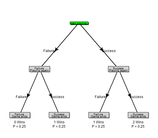
A Bernoulli process is a sequence of Bernoulli trials (the realization of n binary random variables), taking two values (0/1, Heads/Tails, Boy/Girl, etc…). It is often used in teaching introductory probability/statistics classes about the binomial distribution. When visualizing a Bernoulli process, it is common to use a binary tree diagram in order to show the […]

A Bernoulli process is a sequence of Bernoulli trials (the realization of n binary random variables), taking two values (0/1, Heads/Tails, Boy/Girl, etc…). It is often used in teaching introductory probability/statistics classes about the binomial distribution.

When visualizing a Bernoulli process, it is common to use a binary tree diagram in order to show the progression of the process, as well as the various consequences of the trial. We might also include the number of “successes”, and the probability for reaching a specific terminal node.

I wanted to be able to create such a diagram using R. For this purpose I composed some code which uses the {diagram} R package. The final function should allow one to create different sizes of diagrams, while allowing flexibility with regards to the text which is used in the tree.

Here is an example of the simplest use of the function:

source("https://www.r-statistics.com/wp-content/uploads/2011/11/binary.tree_.for_.binomial.game_.r.txt") # loading the function
binary.tree.for.binomial.game(2) # creating a tree for B(2,0.5)

The resulting diagram will look like this:

The same can be done for creating larger trees. For example, here is the code for a 4 stage Bernoulli process:

source("https://www.r-statistics.com/wp-content/uploads/2011/11/binary.tree_.for_.binomial.game_.r.txt") # loading the function
binary.tree.for.binomial.game(4) # creating a tree for B(4,0.5)

The resulting diagram will look like this:

The function can also be tweaked in order to describe a more specific story. For example, the following code describes a 3 stage Bernoulli process where an unfair coin is tossed 3 times (with probability of it giving heads being 0.8):

source("https://www.r-statistics.com/wp-content/uploads/2011/11/binary.tree_.for_.binomial.game_.r.txt") # loading the function

binary.tree.for.binomial.game(3, 0.8, first_box_text = c("Tossing an unfair coin", "(3 times)"), left_branch_text = c("Failure", "Playing again"), right_branch_text = c("Success", "Playing again"),
    left_leaf_text = c("Failure", "Game ends"), right_leaf_text = c("Success",
        "Game ends"), cex = 0.8, rescale_radx = 1.2, rescale_rady = 1.2,
    box_color = "lightgrey", shadow_color = "darkgrey", left_arrow_text = c("Tails n(P = 0.2)"),
    right_arrow_text = c("Heads n(P = 0.8)"), distance_from_arrow = 0.04)

The resulting diagram is:

If you make up neat examples of using the code (or happen to find a bug), or for any other reason – you are welcome to leave a comment.

(note: the images above are licensed under CC BY-SA)

The present and future of the R blogosphere (~7 minute video from useR2011)

This is (roughly) the lightning talk I gave in useR2011. If you are a reader of R-bloggers.com then this talk is not likely to tell you anything new. However, if you have a friend, college or student who is a new useRs of R, this talk will offer him a decent introduction to what the R […]

This is (roughly) the lightning talk I gave in useR2011. If you are a reader of R-bloggers.com then this talk is not likely to tell you anything new. However, if you have a friend, college or student who is a new useRs of R, this talk will offer him a decent introduction to what the R blogosphere is all about.

The talk is a call for people of the R community to participate more in reading, writing and interacting with blogs.

I was encouraged to record this talk per the request of Chel Hee Lee, so it may be used in the recent useR conference in Korea (2011)

The talk (briefly) goes through:

  1. The widespread influence of the R blogosphere
  2. What R bloggers write about
  3. How to encourage a blogger you enjoy reading to keep writing
  4. How to start your own R blog (just go to wordpress.com)
  5. Basic tips about writing a blog
  6. One advice about marketing your R blog (add it to R-bloggers.com)
  7. And two thoughts about the future of R blogging (more bloggers and readers, and more interactive online visualization)

My apologies for any of the glitches in my English. For more talks about R, you can visit the R user groups blog. I hope more speakers from useR 2011 will consider uploading their talks online.

Comparison of ave, ddply and data.table

A guest post by Paul Hiemstra. ———— Fortran and C programmers often say that interpreted languages like R are nice and all, but lack in terms of speed. How fast something works in R greatly depends on how it is implemented, i.e. which packages/functions does one use. A prime example, which shows up regularly on […]

A guest post by Paul Hiemstra.
————

Fortran and C programmers often say that interpreted languages like R are nice and all, but lack in terms of speed. How fast something works in R greatly depends on how it is implemented, i.e. which packages/functions does one use. A prime example, which shows up regularly on the R-help list, is letting a vector grow as you perform an analysis. In pseudo-code this might look like:

1
2
3
4
5
dum = NULL
for(i in 1:100000) {
   # new_outcome = ...do some stuff...
   dum = c(dum, new_outcome)
}

The problem here is that dum is continuously growing in size. This forces the operating system to allocate new memory space for the object, which is terribly slow. Preallocating dum to the length it is supposed to be greatly improves the performance. Alternatively, the use of apply type of functions, or functions from plyr package prevent these kinds of problems. But even between more advanced methods there are large differences between different implementations.

Take the next example. We create a dataset which has two columns, one column with values (e.g. amount of rainfall) and in the other a category (e.g. monitoring station id). We would like to know what the mean value is per category. One way is to use for loops, but I’ll skip that one for now. Three possibilities exist that I know of: ddply (plyr), ave (base R) and data.table. The piece of code at the end of this post compares these three methods. The outcome in terms of speed is:
(press the image to see a larger version)

1
2
3
4
5
6
7
8
9
10
11
12
13
14
15
16
17
   datsize noClasses  tave tddply tdata.table
1    1e+05        10 0.091  0.035       0.011
2    1e+05        50 0.102  0.050       0.012
3    1e+05       100 0.105  0.065       0.012
4    1e+05       200 0.109  0.101       0.010
5    1e+05       500 0.113  0.248       0.012
6    1e+05      1000 0.123  0.438       0.012
7    1e+05      2500 0.146  0.956       0.013
8    1e+05     10000 0.251  3.525       0.020
9    1e+06        10 0.905  0.393       0.101
10   1e+06        50 1.003  0.473       0.100
11   1e+06       100 1.036  0.579       0.105
12   1e+06       200 1.052  0.826       0.106
13   1e+06       500 1.079  1.508       0.109
14   1e+06      1000 1.092  2.652       0.111
15   1e+06      2500 1.167  6.051       0.117
16   1e+06     10000 1.338 23.224       0.132

It is quite obvious that ddply performs very bad when the number of unique categories is large. The ave function performs better. However, the data.table option is by far the best one, outperforming both other alternatives easily. In response to this, Hadley Wickham (author of plyr) responded:

This is a drawback of the way that ddply always works with data frames. It will be a bit faster if you use summarise instead of data.frame (because data.frame is very slow), but I’m still thinking about how to overcome this fundamental limitation of the ddply approach.

I hope this comparison is of use to readers. And remember, think before complaining that R is slow :) .

Paul (e-mail: [email protected])

ps This blogpost is based on discussions on the R-help and manipulatr mailing lists:
http://www.mail-archive.com/[email protected]/msg142797.html
http://groups.google.com/group/manipulatr/browse_thread/thread/5e8dfed85048df99

R code to perform the comparison

1
2
3
4
5
6
7
8
9
10
11
12
13
14
15
16
17
18
19
20
21
22
library(ggplot2)
library(data.table)
theme_set(theme_bw())
datsize = c(10e4, 10e5)
noClasses = c(10, 50, 100, 200, 500, 1000, 2500, 10e3)
comb = expand.grid(datsize = datsize, noClasses = noClasses)
res = ddply(comb, .(datsize, noClasses), function(x) {
  expdata = data.frame(value = runif(x$datsize),
                      cat = round(runif(x$datsize, min = 0, max = x$noClasses)))
  expdataDT = data.table(expdata)
 
  t1 = system.time(res1 <- with(expdata, ave(value, cat)))
  t2 = system.time(res2 <- ddply(expdata, .(cat), mean))
  t3 = system.time(res3 <- expdataDT[, sum(value), by = cat])
  return(data.frame(tave = t1[3], tddply = t2[3], tdata.table = t3[3]))
}, .progress = 'text')
 
res
 
ggplot(aes(x = noClasses, y = log(value), color = variable), data =
melt(res, id.vars = c("datsize","noClasses"))) + facet_wrap(~ datsize)
+ geom_line()

Calling R lovers and bloggers – to work together on "The R Programming wikibook"

This post is a call for both R community members and R-bloggers, to come and help make The R Programming wikibook be amazing.

The R Programming wikibook is not just another one of the many free books about statistics/R, it is a community project which aims to create a cross-disciplinary practical guide to the R programming language.  Here is how you can join:

Continue reading “Calling R lovers and bloggers – to work together on "The R Programming wikibook"”

Engineering Data Analysis (with R and ggplot2) – a Google Tech Talk given by Hadley Wickham

It appears that just days ago, Google Tech Talk released a new, one hour long, video of a presentation (from June 6, 2011) made by one of R’s community more influential contributors, Hadley Wickham.

This seems to be one of the better talks to send a programmer friend who is interested in getting into R.

Talk abstract

Data analysis, the process of converting data into knowledge, insight and understanding, is a critical part of statistics, but there’s surprisingly little research on it. In this talk I’ll introduce some of my recent work, including a model of data analysis. I’m a passionate advocate of programming that data analysis should be carried out using a programming language, and I’ll justify this by discussing some of the requirement of good data analysis (reproducibility, automation and communication). With these in mind, I’ll introduce you to a powerful set of tools for better understanding data: the statistical programming language R, and the ggplot2 domain specific language (DSL) for visualisation.

The video

More resources

How to upgrade R on windows 7

Background – time to upgrade to R 2.13.0

The news of the new release of R 2.13.0 is out, and the R blogosphere is buzzing. Bloggers posting excitedly about the new R compiler package that brings with it the hope to speed up our R code with up to 4 times improvement and even a JIT compiler for R. So it is time to upgrade, and bloggers are here to help. Some wrote how to upgrade R on Linux and mac OSX (based on posts by Paolo). And it is now my turn, with suggestions on how to upgrade R on windows 7.

Upgrading R on windows – the two strategies

The classic description of how to upgrade R can be found in the R project FAQ page (and also the FAQ on how to install R on windows)

There are basically two strategies for R upgrading on windows. The first is to install a new R version and copy paste all the packages to the new R installation folder. The second is to have a global R package folder, each time synced to the most current R installation (thus saving us the time of copying the package library each we upgrade R).

I described the second strategy in detail in a post I wrote a year ago titled: “How to upgrade R on windows XP – another strategy” which explains how to upgrade R using the simple two-liner code:

source("https://www.r-statistics.com/wp-content/uploads/2010/04/upgrading-R-on-windows.r.txt")
New.R.RunMe()

p.s: If this is the first time you are upgrading R using this method, then first run the following two lines on your old R installation (before running the above code in the new R intallation):

source("https://www.r-statistics.com/wp-content/uploads/2010/04/upgrading-R-on-windows.r.txt")
Old.R.RunMe()

The above code should be enough.  However, there are some common pitfalls you might encounter when upgrading R on windows 7, bellow I outline the ones I know about, and how they can be solved.

Continue reading “How to upgrade R on windows 7”

Article about plyr published in JSS, and the citation was added to the new plyr (version 1.5)

The plyr package (by Hadley Wickham) is one of the few R packages for which I can claim to have used for all of my statistical projects. So whenever a new version of plyr comes out I tend to be excited about it (as was when version 1.2 came out with support for parallel processing)

So it is no surprise that the new release of plyr 1.5 got me curious. While going through the news file with the new features and bug fixes, I noticed how (quietly) Hadley has also released (6 days ago) another version of plyr prior to 1.5 which was numbered 1.4.1. That version included only one more function, but a very important one – a new citation reference for when using the plyr package. Here is how to use it:

install.packages("plyr") # so to upgrade to the latest release
citation("plyr")

The output gives both a simple text version as well as a BibTeX entry for LaTeX users. Here it is (notice the download link for yourself to read):

To cite plyr in publications use:
Hadley Wickham (2011). The Split-Apply-Combine Strategy for Data
Analysis. Journal of Statistical Software, 40(1), 1-29. URL
http://www.jstatsoft.org/v40/i01/.

I hope to see more R contributers and users will make use of the ?citation() function in the future.

Beeswarm Boxplot (and plotting it with R)

2016-05-28 update: I strongly recommend reading the comment by Leland Wilkinson. In summary, “beeswarm” plots are not recommended as they often create visual artifacts that distracts from the estimated density of the observations.

fig_05

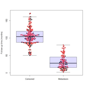
(The image above is called a “Beeswarm Boxplot” , the code for producing this image is provided at the end of this post)

The above plot is implemented under different names in different softwares. This “Scatter Dot Beeswarm Box Violin – plot” (in the lack of an agreed upon term) is a one-dimensional scatter plot which is like “stripchart”, but with closely-packed, non-overlapping points; the positions of the points are corresponding to the frequency in a similar way as the violin-plot. The plot can be superimposed with a boxplot to give a very rich description of the underlaying distribution.

This plot has been implemented in various statistical packages, in this post I will list the few I came by so far. And if you know of an implementation I’ve missed please tell me about it in the comments.

Continue reading “Beeswarm Boxplot (and plotting it with R)”