Tailor Your Tables with stargazer: New Features for LaTeX and Text Output

Guest post by Marek Hlavac

Since its first introduction on this blog, stargazer, a package for turning R statistical output into beautiful LaTeX and ASCII text tables, has made a great deal of progress. Compared to available alternatives (such as apsrtable or texreg), the latest version (4.0) of stargazer supports the broadest range of model objects. In particular, it can create side-by-side regression tables from statistical model objects created by packages AER, betareg, dynlm, eha, ergm, gee, gmm, lme4, MASS, mgcv, nlme, nnet, ordinal, plm, pscl, quantreg, relevent, rms, robustbase, spdep, stats, survey, survival and Zelig.  You can install stargazer from CRAN in the usual way:

install.packages(“stargazer”)

New Features: Text Output and Confidence Intervals

In this blog post, I would like to draw attention to two new features of stargazer that make the package even more useful:

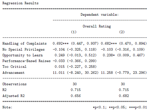
  • stargazer can now produce ASCII text output, in addition to LaTeX code. As a result, users can now create beautiful tables that can easily be inserted into Microsoft Word documents, published on websites, or sent via e-mail. Sharing your regression results has never been easier. Users can also use this feature to preview their LaTeX tables before they use the stargazer-generated code in their .tex documents.
  • In addition to standard errors, stargazer can now report confidence intervals at user-specified confidence levels (with a default of 95 percent). This possibility might be especially appealing to researchers in public health and biostatistics, as the reporting of confidence intervals is very common in these disciplines.

In the reproducible example presented below, I demonstrate these two new features in action.


Reproducible Example

I begin by creating model objects for two Ordinary Least Squares (OLS) models (using the lm() command) and a probit model (using glm() ). Note that I use data from attitude, one of the standard data frames that should be provided with your installation of R.

## 2 OLS models

linear.1 <- lm(rating ~ complaints + privileges + learning + raises + critical, data=attitude)
linear.2 <- lm(rating ~ complaints + privileges + learning, data=attitude)

## create an indicator dependent variable, and run a probit model

attitude$high.rating <- (attitude$rating > 70)
probit.model <- glm(high.rating ~ learning + critical + advance, data=attitude, family = binomial(link = "probit"))

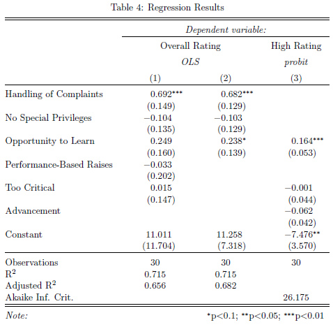
I then use stargazer to create a ‘traditional’ LaTeX table with standard errors. With the sole exception of the argument no.space – which I use to save space by removing all empty lines in the table – both the command call and the resulting table should look familiar from earlier versions of the package:

stargazer(linear.1, linear.2, probit.model, title="Regression Results", align=TRUE, dep.var.labels=c("Overall Rating","High Rating"), covariate.labels=c("Handling of Complaints","No Special Privileges", "Opportunity to Learn","Performance-Based Raises","Too Critical","Advancement"), omit.stat=c("LL","ser","f"), no.space=TRUE)

table_example_1

Continue reading "Tailor Your Tables with stargazer: New Features for LaTeX and Text Output"
{stargazer} package for beautiful LaTeX tables from R statistical models output

stargazer is a new R package that creates LaTeX code for well-formatted regression tables, with multiple models side-by-side, as well as for summary statistics tables. It can also output the content of data frames directly into LaTeX. Compared to available alternatives, stargazer excels in three regards:  its ease of use, the large number of models it supports, and its beautiful aesthetics.

Ease of use

stargazer was designed with the user’s comfort in mind. The learning curve is very mild and all arguments are very intuitive, so that even a beginning user of R or LaTeX can quickly become familiar with the package’s many capabilities. The package is intelligent, and tries to minimize the amount of effort the user has to put into adjusting argument values. If stargazer is given a set of regression model objects, for instance, the package will create a side-by-side regression table. By contrast, if the user feeds it a data frame, stargazer will know that the user is most likely looking for a summary statistics table or – if the summary argument is set to false – wants to output the content of the data frame.

A quick reproducible example shows just how easy stargazer is to use. You can install stargazer from CRAN in the usual way:

install.packages("stargazer")
library(stargazer)

Continue reading “{stargazer} package for beautiful LaTeX tables from R statistical models output”

Printing nested tables in R – bridging between the {reshape} and {tables} packages

This post shows how to print a prettier nested pivot table, created using the {reshape} package (similar to what you would get with Microsoft Excel), so you could print it either in the R terminal or as a LaTeX table. This task is done by bridging between the cast_df object produced by the {reshape} package, […]

This post shows how to print a prettier nested pivot table, created using the {reshape} package (similar to what you would get with Microsoft Excel), so you could print it either in the R terminal or as a LaTeX table. This task is done by bridging between the cast_df object produced by the {reshape} package, and the tabular function introduced by the new {tables} package.

Here is an example of the type of output we wish to produce in the R terminal:

1
2
3
4
5
6
7
       ozone       solar.r        wind         temp
 month mean  sd    mean    sd     mean   sd    mean  sd
 5     23.62 22.22 181.3   115.08 11.623 3.531 65.55 6.855
 6     29.44 18.21 190.2    92.88 10.267 3.769 79.10 6.599
 7     59.12 31.64 216.5    80.57  8.942 3.036 83.90 4.316
 8     59.96 39.68 171.9    76.83  8.794 3.226 83.97 6.585
 9     31.45 24.14 167.4    79.12 10.180 3.461 76.90 8.356

Or in a latex document:

Motivation: creating pretty nested tables

In a recent post we learned how to use the {reshape} package (by Hadley Wickham) in order to aggregate and reshape data (in R) using the melt and cast functions.

The cast function is wonderful but it has one problem – the format of the output. As opposed to a pivot table in (for example) MS excel, the output of a nested table created by cast is very “flat”. That is, there is only one row for the header, and only one column for the row names. So for both the R terminal, or an Sweave document, when we deal with a more complex reshaping/aggregating, the result is not something you would be proud to send to a journal.

The opportunity: the {tables} package

The good news is that Duncan Murdoch have recently released a new package to CRAN called {tables}. The {tables} package can compute and display complex tables of summary statistics and turn them into nice looking tables in Sweave (LaTeX) documents. For using the full power of this package, you are invited to read through its detailed (and well written) 23 pages Vignette. However, some of us might have preferred to keep using the syntax of the {reshape} package, while also benefiting from the great formatting that is offered by the new {tables} package. For this purpose, I devised a function that bridges between cast_df (from {reshape}) and the tabular function (from {tables}).

The bridge: between the {tables} and the {reshape} packages

The code for the function is available on my github (link: tabular.cast_df.r on github) and it seems to works fine as far as I can see (though I wouldn’t run it on larger data files since it relies on melting a cast_df object.)

Here is an example for how to load and use the function:

1
2
3
4
5
6
7
8
9
10
11
12
13
14
15
16
17
18
19
20
21
22
23
24
25
26
27
28
29
30
31
32
33
34
######################
# Loading the functions
######################
# Making sure we can source code from github
source("https://www.r-statistics.com/wp-content/uploads/2012/01/source_https.r.txt")
 
# Reading in the function for using tabular on a cast_df object:
source_https("https://raw.github.com/talgalili/R-code-snippets/master/tabular.cast_df.r")


######################
# example:
######################
 
############
# Loading and preparing some data
require(reshape)
names(airquality) <- tolower(names(airquality))
airquality2 <- airquality
airquality2$temp2 <- ifelse(airquality2$temp > median(airquality2$temp), "hot", "cold")
aqm <- melt(airquality2, id=c("month", "day","temp2"), na.rm=TRUE)
colnames(aqm)[4] <- "variable2"	# because otherwise the function is having problem when relying on the melt function of the cast object
head(aqm,3)
#  month day temp2 variable2 value
#1     5   1  cold     ozone    41
#2     5   2  cold     ozone    36
#3     5   3  cold     ozone    12
 
############
# Running the example:
tabular.cast_df(cast(aqm, month ~ variable2, c(mean,sd)))
tabular(cast(aqm, month ~ variable2, c(mean,sd))) # notice how we turned tabular to be an S3 method that can deal with a cast_df object
Hmisc::latex(tabular(cast(aqm, month ~ variable2, c(mean,sd)))) # this is what we would have used for an Sweave document

And here are the results in the terminal:

1
2
3
4
5
6
7
8
9
10
11
12
13
14
15
16
17
18
19
>
> tabular.cast_df(cast(aqm, month ~ variable2, c(mean,sd)))
 
       ozone       solar.r        wind         temp
 month mean  sd    mean    sd     mean   sd    mean  sd
 5     23.62 22.22 181.3   115.08 11.623 3.531 65.55 6.855
 6     29.44 18.21 190.2    92.88 10.267 3.769 79.10 6.599
 7     59.12 31.64 216.5    80.57  8.942 3.036 83.90 4.316
 8     59.96 39.68 171.9    76.83  8.794 3.226 83.97 6.585
 9     31.45 24.14 167.4    79.12 10.180 3.461 76.90 8.356
> tabular(cast(aqm, month ~ variable2, c(mean,sd))) # notice how we turned tabular to be an S3 method that can deal with a cast_df object
 
       ozone       solar.r        wind         temp
 month mean  sd    mean    sd     mean   sd    mean  sd
 5     23.62 22.22 181.3   115.08 11.623 3.531 65.55 6.855
 6     29.44 18.21 190.2    92.88 10.267 3.769 79.10 6.599
 7     59.12 31.64 216.5    80.57  8.942 3.036 83.90 4.316
 8     59.96 39.68 171.9    76.83  8.794 3.226 83.97 6.585
 9     31.45 24.14 167.4    79.12 10.180 3.461 76.90 8.356

And in an Sweave document:

Here is an example for the Rnw file that produces the above table:
cast_df to tabular.Rnw

I will finish with saying that the tabular function offers more flexibility then the one offered by the function I provided. If you find any bugs or have suggestions of improvement, you are invited to leave a comment here or inside the code on github.

(Link-tip goes to Tony Breyal for putting together a solution for sourcing r code from github.)